Greenhouse Gas Protocols: Understanding Scope 3 Emissions

Climate Science and the Scopes of GHG Emissions

One of the most widely understood aspects of climate change is the effect that greenhouse gases in the atmosphere have on the temperature regulation of Earth. Greenhouse gas (GHG) emissions are compounds such as carbon dioxide (CO2) and methane (CH4) that are released as biproducts of reactions caused by the systemic processes of producing energy, waste, transportation, manufacturing, and agriculture. These and other GHG compounds capture energy from the Sun, thus trapping heat and emissions within the atmosphere and warming the earth at an unnatural rate. The drastic increase of greenhouse gases began in the late 19^ה' century with the rapid scale of industrialization, catalyzing a major shift in global ecology known as climate change.

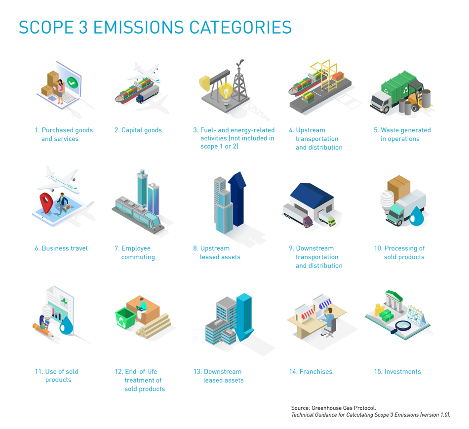
Emissions tracking is an important area of climate science that helps direct climate action on an institutional scale. These emissions sources have been split into Scopes 1, 2, and 3, which respectively encompass: emissions directly from the institution’s facilities or vehicle (Scope 1), emissions sourced from purchased electricity (Scope 2), and the indirect emissions associated with running an institution (Scope 3). This range covers fifteen categories of industry and accounts for upstream and downstream emissions from capital goods produced, services rendered, institutional investments, visitor travel, staff commuting, transportation and distribution, waste generated from operations, and raw materials extraction.

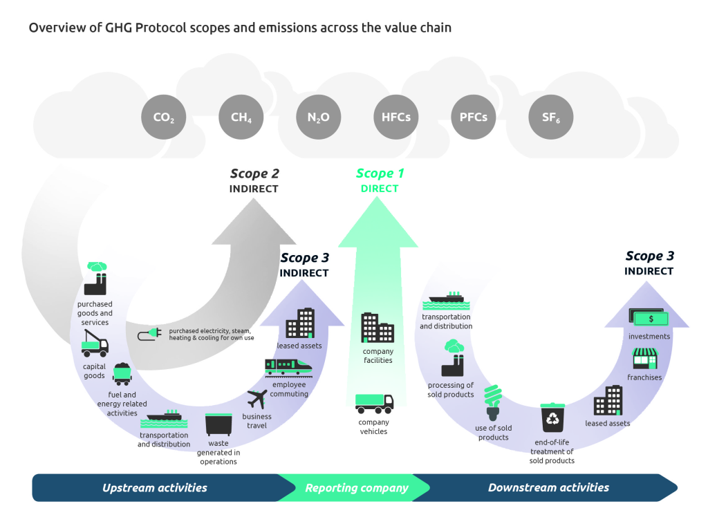
Scopes 1 and 2 are focused on production of energy and account for around 73% of total GHG emissions. Conversely, Scope 3 emissions represent the broadest category of possible emissions and is an underrepresented area of climate action. Outside of climate-conscious fields, Scope 3 is not often known because quantifying emissions from areas that are not directly associated with on-campus operations of an organization can be a difficult task.

Scope 3 is an interesting area for further research, as it can be broad and difficult to constrain, and even more difficult to quantify. A good analogy for Scope 3 emissions is that of a river. Rain falls on a hill and eventually channelizes into rivulets, which conjoin and grow into a full-sized river. It is easy to see the river as a whole, but difficult to count all the tributary streams, creeks, and rivulets. It is even more difficult to quantify the overland flow before any channelization occurs. For Scope 3 emissions, it is far easier to consider the emissions for shipping food and merchandise than it is to look at the energy costs of fabricating the plastic packaging that food is served in, the emissions released by the tractors used to farm the land that grew the lettuce for salads, and the land costs for farming the feed that produce the meat that is on the menu.

What Do We Measure?

Creation of a GHG inventory is an important step for any organization that is quantifying Scope 3 emissions, moving toward higher levels of accountability in the supply chain, and improving institutional climate consciousness. The process of compiling a GHG inventory involves setting the scope by giving a concrete time frame of tracking, identifying aspects of operations as sources for consideration – such as supply chains, investments, or travel – and determining the specific GHGs that will be tracked.

Much of the difficulty in tracking Scope 3 emissions is in the non-mandatory reporting of emissions in a few key sectors. Therefore, calculations of Scope 3 tend to rely heavily on secondary emissions tracking sources and more generalized models. These calculations are often performed by outside consultants who specialize in tracking Scope 3 emissions. Calculating emissions in this way leaves room for errors such as double counting, missing areas, and under or over estimation. Consultants often make decisions to leave certain fields that may obfuscate the calculations out of emissions tracking.

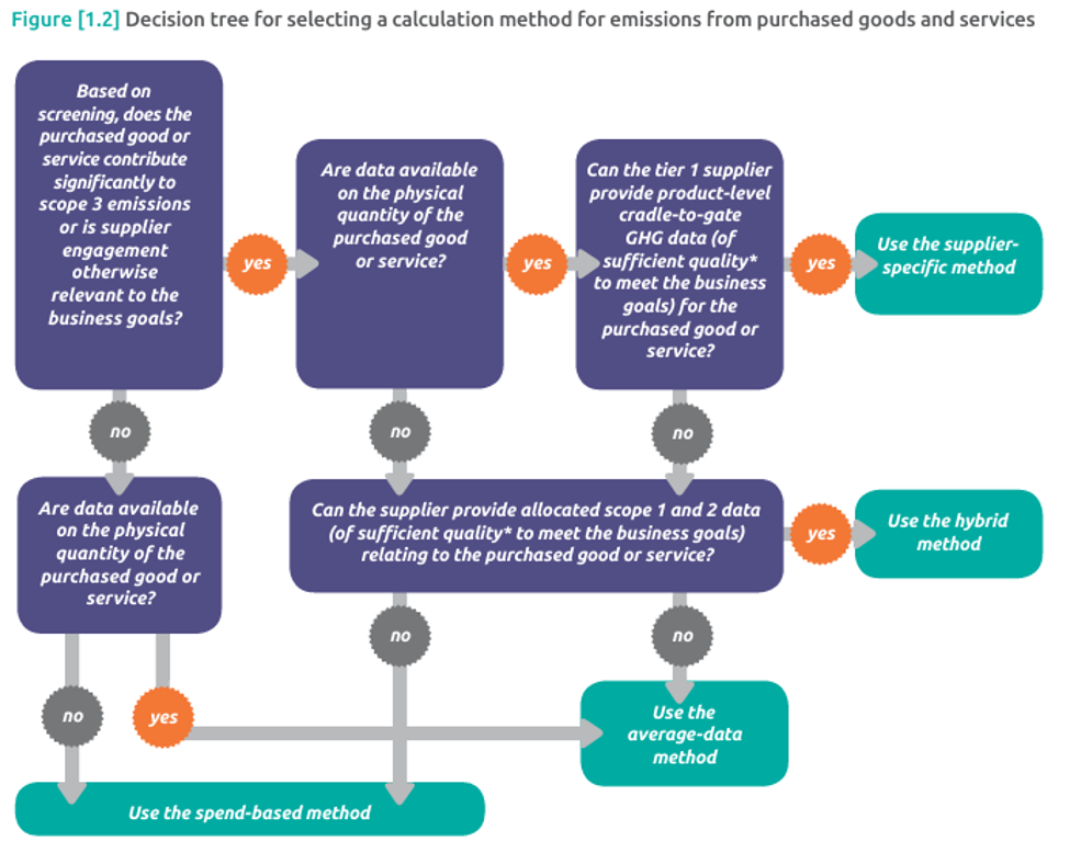
Because of these difficulties with quantifying certain emissions, it is important to limit the scope of emissions reporting to areas that are actionable on institutional and individual levels, high spending, and have the possibility for reduction. For example, Yale Sustainability identified IT hardware, building materials, and food services as areas of high interest for Scope 3 emissions reporting, while inspections, insurance, and taxes are less actionable areas. Calculation of Scope 3 emissions can be a game of balancing how much can be calculated for broad areas versus how much guesswork has to go into calculating specific emissions.

Calculating Scope 3 emissions is comparable to the coastline paradox whereas you measure the shoreline of an island, its perimeter appears to increase as you refine the scale to be more precise. In terms of Scope 3, as we become able to more rigorously track emissions, it appears that there are more emissions that were unaccounted for. However, this is a part of the paradox, as these emissions have always existed for these fields, but only by tracking them do we see how much they have been contributing to the total sum of emissions for an institution. By limiting the scale of the measurements we make, we focus on actionable areas that can reduce emissions.

Scope 3 emissions are calculated in measures of equivalent warming potential to carbon dioxide. Different gases last for different lengths of time in the atmosphere and reflect different amounts of sunlight. Since it can be difficult to quantify this in different units, a conversion factor is used. This factor is called Global Warming Potential (GWP) and describes the amount of harm a unit of any greenhouse gas does over a one-hundred-year timeframe when compared to one unit of CO₂. The compound methane (CH₄) has a factor of 28, while the group of compounds hydrofluorocarbons (HFCs) have variable GWP from 4,000 to 12,000. To put this into perspective, a 1-kilogram leak in a refrigeration unit that uses HFCs could be equivalent to up to 12,000 kilograms of direct CO₂ emissions. This is another reason why Scope 3 emissions reporting can be difficult to fully quantify; having to consider conversion factors of many different gases is why an inventory of GHGs is one of the strongest ways to begin calculating and reporting of Scope 3 emissions.

Source: Caretakers of Wonder Partner Action Plans

Partners Taking Action

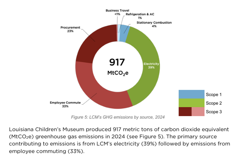
There are examples of cultural institutions actively measuring and reducing Scope 3 emissions. Check out the Caretakers of Wonder initiative to read about the work being conducted by The Wild Center, Louisiana Children’s Museum, Chicago Children’s Museum, The Children’s Museum of Southern Oregon, and Museum of Discovery + Science; or read The Climate Toolkit’s spotlight feature with Denver Zoo to explore unique zoological categories of Scope 3 emissions such as animal transport, waste, and nutrition procurement. If you’re looking for tools to help your institution get started with identifying and measuring emissions, check out Greenhouse Gas Protocol’s Technical Guidance for Calculating Scope 3 Emissions.

Scope 3 emissions are an underrepresented, but not unconsidered, area of climate research. There has been increasing desire to understand and limit Scope 3 in recent years as we learn more about the interconnectivity of economy and industry, the ripple-effects of our institutional actions, and how they’ve affected our changing climate.